Week 3. FREQUENCY DISTRIBUTIONS: In-Class Practice
Yuriy Davydenko
May 11, 2020
Download the datasets for this class:
You can download this whole script as week03.Rmd file to save on your computer and open in RStudio instead of copying & pasting from this webpage:
For those who prefer to work with RCloud, a project with the same materials, including Computer Assignment 2, can be accessed using the following link:
#install.packages("dplyr")   # install packages if they are not installed yet
#install.packages("ggplot2") # (uncomment the command before executing it by removing '#' in front of it)
#install.packages("knitr")
#install.packages("summarytools")

library(dplyr)         # for manipulating data
library(ggplot2)       # for making graphs
library(knitr)         # for nicer table formatting
library(summarytools)  # for frequency distribution tables
3.1 Frequency Distribution Tables
(See Lecture Notes for Week 3 on iCollege to read about interpreting frequency tables)
Example 1: Two sets of rated charities
Assume you are studying charitable performance and have two samples of charities - one sample of 10 charities “Datasets/s10.RData” and one sample of 100 charities. Each sample contains data on charity ratings. Let’s read the datasets into R and generate frequency tables for each ssample:
load("Datasets/s10.RData")   # load charity ratings data: the sample of 10
freq(s10)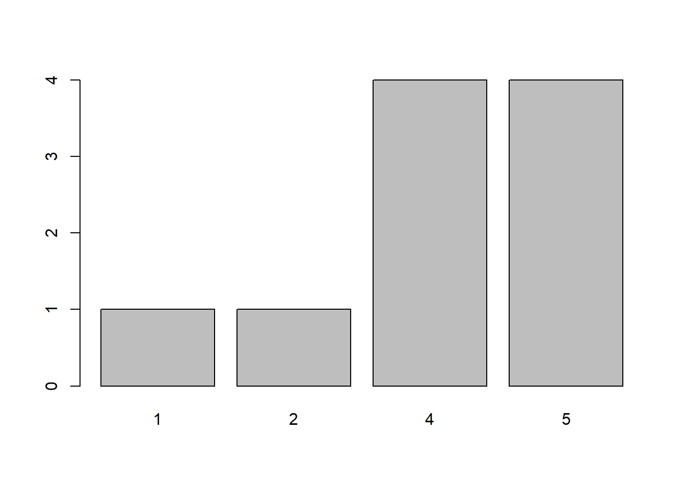
## s10
##       Frequency Percent
## 1             1      10
## 2             1      10
## 4             4      40
## 5             4      40
## Total        10     100
load("Datasets/s100.RData") # load charity ratings data: the sample of 100
freq(s100)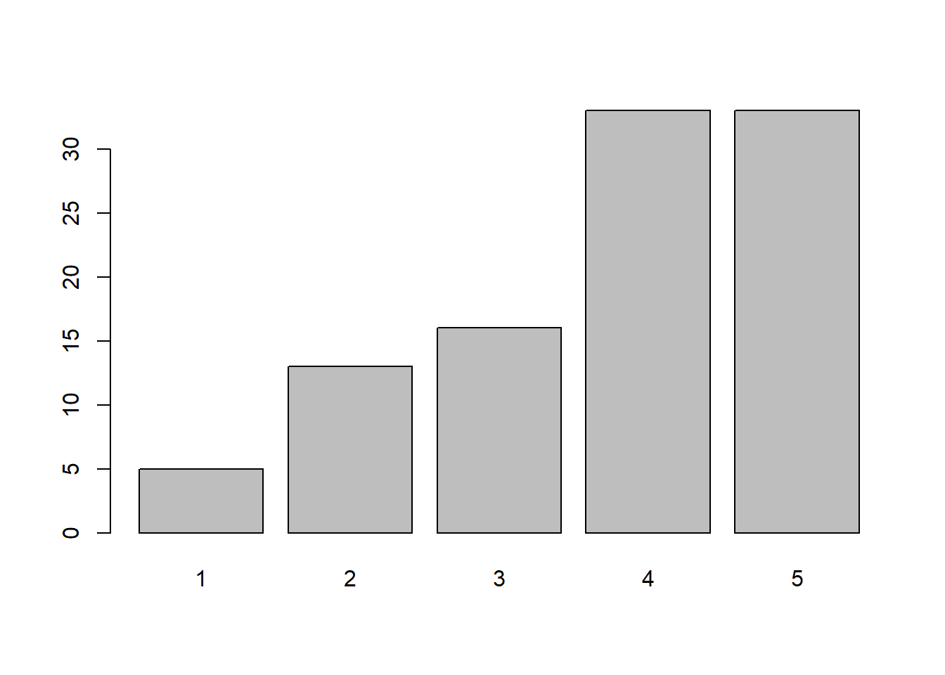
## s100
##       Frequency Percent
## 1             5       5
## 2            13      13
## 3            16      16
## 4            33      33
## 5            33      33
## Total       100     100
EXAMPLE 2: General Social Survey (GSS)
Assume you are studying Americans’ attitudes toward premarital sex. In 1998, the General Social Survey (GSS) asked a random sample of Americans, the following question:
There’s been a lot of discussion about the way morals and attitudes about sex are changing in this country. If a man and woman have sex relations before marriage, do you think it is always wrong, almost always wrong, wrong only sometimes, or not wrong at all?
We have a sample with 1000 responses to some of the survey questions, including the question about respondents’ attitudes toward sex before marriage.
Let’s load the dataset gss98_4041.csv from the Dataset folder:
load(file = "Datasets/gss98.RData")The dataset contains data on the following 49 variables:
names(gss98)## [1] "X.1" "X" "SEX" "RACE" "RELIG" "FUND"
## [7] "MARITAL" "ATTEND" "PREMARSX" "XMARSEX" "HOMOSEX" "TEENSEX"
## [13] "ABANY" "CAPPUN" "GUNLAW" "GRASS" "PRAYER" "NATCITY"
## [19] "NATHEAL" "NATCRIME" "NATDRUG" "NATEDUC" "NATRACE" "NATFARE"
## [25] "NATROAD" "NATMASS" "CONCLERG" "CONEDUC" "CONFED" "CONPRESS"
## [31] "CONJUDGE" "CONLEGIS" "FECHLD" "FEHELP" "FEPRESCH" "FEFAM"
## [37] "RACDIF1" "LIVEBLKS" "MARBLK" "DISCAFF" "PARTY" "IDEOLOGY"
## [43] "AGESUM" "INCOME" "EDUC2" "REGION2" "CITY" "RURAL"
## [49] "PROT" "NEWFUND"To learn more about each variable see the codebook for the survey here.
Let’s take a look at several selected Variables (first ten cases) from the General Social Survey (GSS) 1998:
gss98[1:10, c("SEX", "RACE", "RELIG", "AGESUM", "EDUC2", "FUND", "MARITAL", "INCOME", "PARTY", "PREMARSX")] %>% kable()| SEX | RACE | RELIG | AGESUM | EDUC2 | FUND | MARITAL | INCOME | PARTY | PREMARSX |
|---|---|---|---|---|---|---|---|---|---|
| male | White | Protestant | 30 to 44 | high school graduate | liberal | Married | $60,000 or more | Independent | Always wrong |
| male | White | Catholic | 18 to 29 | high school graduate | moderate | Never married | $35,000 to $59,000 | Republican | Not wrong at all |
| female | White | Protestant | 30 to 44 | some college | fundamentalist | Divorced | $20,000 to $34,999 | Democrat | NA |
| female | Other | Catholic | 30 to 44 | less than h.s. diploma | moderate | Widowed | NA | Independent | NA |
| male | White | Protestant | 30 to 44 | college graduate | fundamentalist | Married | $60,000 or more | Republican | NA |
| male | White | Protestant | 60 or older | college graduate | fundamentalist | Married | NA | Independent | Always wrong |
| female | White | Protestant | 30 to 44 | some college | moderate | Never married | NA | Independent | NA |
| female | White | Protestant | 60 or older | some college | liberal | Divorced | $20,000 to $34,999 | Republican | NA |
| male | White | Protestant | 45 to 59 | college graduate | liberal | Divorced | NA | Republican | NA |
| male | White | Protestant | 60 or older | high school graduate | fundamentalist | Married | NA | Independent | Not wrong at all |
[ VAR: PREMARSX ]
According to the survey’s codebook, the variable of interest describing individual attitudes toward premarital sex is labelled PREMARSX.
Let’s generate the Frequency Distribution Table for PREMARSX using the function summarytools::freq('_Variable Name_'):
library(summarytools)   # Make sure you've loaded the library 'summarytools'
gss98$PREMARSX <- factor(gss98$PREMARSX, levels = c("Always wrong", "Almst alwys wrng", "Wrong sometimes", "Not wrong at all"))
freq(gss98$PREMARSX)    # Generate frequency distribution using command 'freq()' from the library 'summarytools'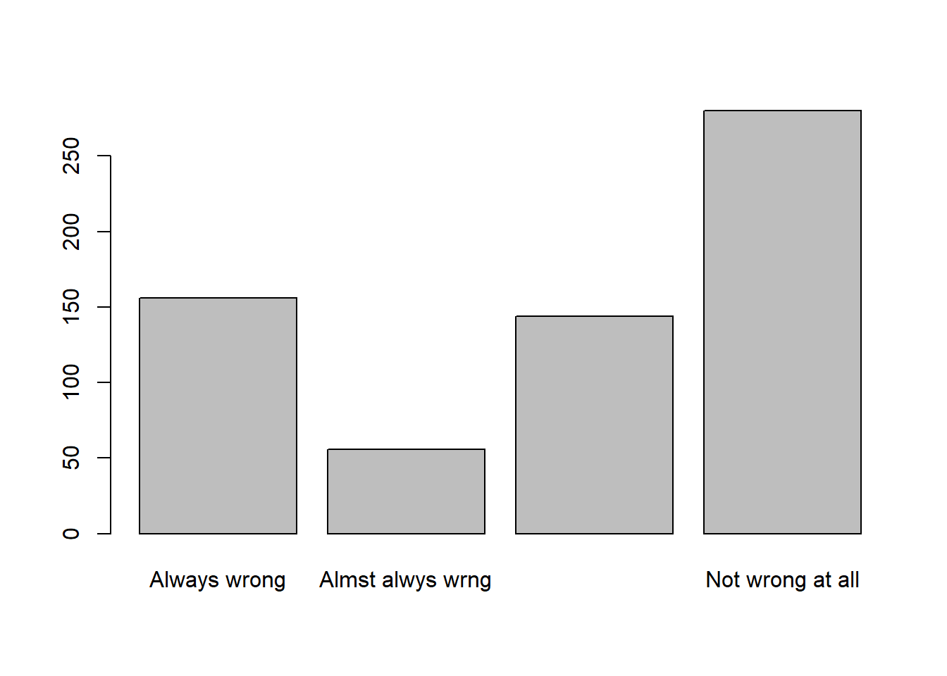
## gss98$PREMARSX
##                  Frequency Percent Valid Percent
## Always wrong           156    15.6        24.528
## Almst alwys wrng        56     5.6         8.805
## Wrong sometimes        144    14.4        22.642
## Not wrong at all       280    28.0        44.025
## NA's                   364    36.4
## Total                 1000   100.0       100.000
Let’s generate frequency tables for two more variables:
[ VAR: HOMOSEX ] What about sexual relations between two adults of the same sex–do you think it is always wrong, almost always wrong, wrong only sometimes, or not wrong at all?
freq(gss98$HOMOSEX)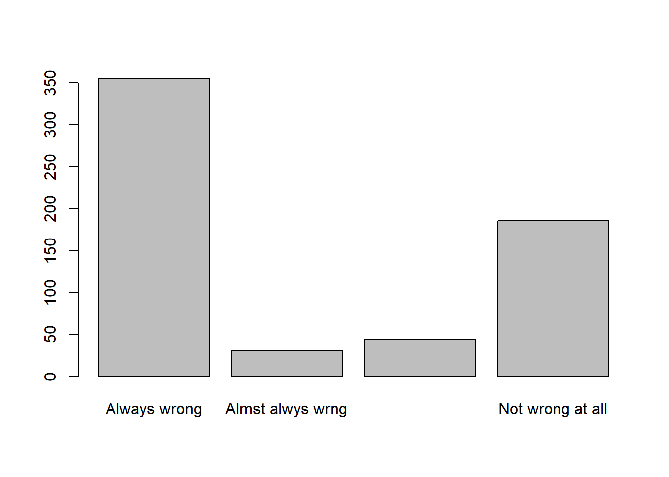
## gss98$HOMOSEX
##                  Frequency Percent Valid Percent
## Always wrong           356    35.6        57.699
## Almst alwys wrng        31     3.1         5.024
## Wrong sometimes         44     4.4         7.131
## Not wrong at all       186    18.6        30.146
## NA's                   383    38.3
## Total                 1000   100.0       100.000
[ VAR: TEENSEX ] What if they are in their early teens, say 14 to 16 years old? In that case, do you think sex relations before marriage are always wrong, almost always wrong, wrong only sometimes, or not wrong at all?
freq(gss98$TEENSEX)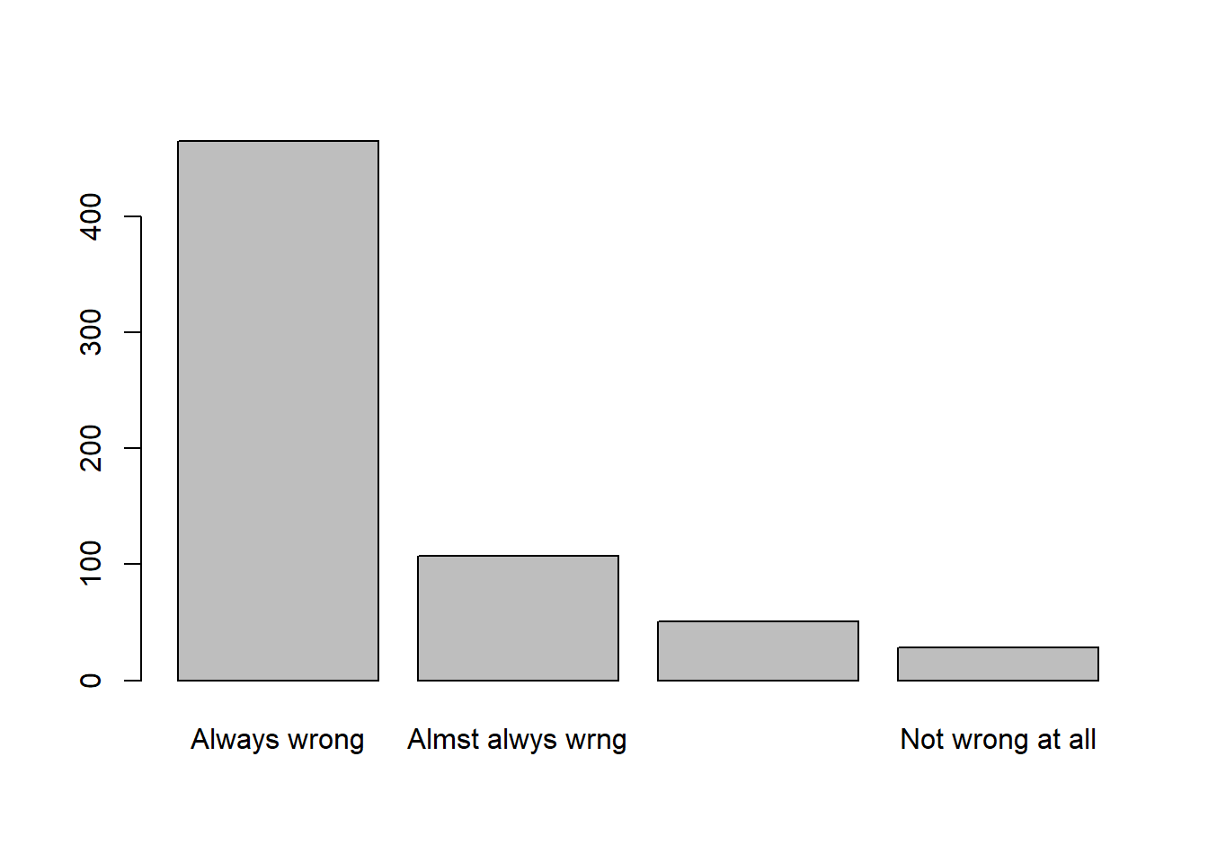
## gss98$TEENSEX
##                  Frequency Percent Valid Percent
## Always wrong           465    46.5        71.429
## Almst alwys wrng       107    10.7        16.436
## Wrong sometimes         51     5.1         7.834
## Not wrong at all        28     2.8         4.301
## NA's                   349    34.9
## Total                 1000   100.0       100.000
EXAMPLE 3: Student Test Scores
Let’s read the dataset with student test scores into R and print the scores on the screen:
test_scores <- read.csv("Datasets/TestScores.csv")
data.frame("Class 1" = test_scores[test_scores$Class=="Class1" , "Score"],
           "Class 2" = test_scores[test_scores$Class=="Class2" , "Score"],
"Class 3" = test_scores[test_scores$Class=="Class3" , "Score"] ) %>% kable(align = c("l","l","l"))| Class.1 | Class.2 | Class.3 |
|---|---|---|
| 79 | 75 | 100 |
| 75 | 78 | 80 |
| 82 | 82 | 93 |
| 91 | 88 | 85 |
| 88 | 92 | 90 |
| 78 | 56 | 70 |
| 79 | 85 | 72 |
| 75 | 90 | 77 |
| 78 | 78 | 79 |
| 0 | 81 | 81 |
| 74 | 79 | 80 |
| 77 | 64 | 82 |
| 81 | 67 | 77 |
| 90 | 41 | 78 |
| 74 | 40 | 92 |
| 71 | 61 | 98 |
| 85 | 68 | 83 |
| 65 | 79 | 83 |
| 73 | 89 | 92 |
| 81 | 64 | 79 |
| 77 | 97 | 80 |
| 74 | 95 | 71 |
| 85 | 73 | 94 |
| 15 | 91 | 92 |
| 82 | 56 | 79 |
| 79 | 64 | 83 |
| 18 | 74 | 81 |
| 32 | 67 | 98 |
| 95 | 67 | 73 |
| 77 | 54 | 91 |
| 83 | 97 | 74 |
| 74 | 87 | 84 |
| 76 | 80 | 91 |
| 60 | 89 | 88 |
| 61 | 81 | 89 |
Let’s generate a contingency table:
testscores <- read.csv("Datasets/TestScores.csv")
summarytools::freq(testscores$Score)                 #Oops, NOT VERY USEFUL !!!
## Frequencies
##
## Freq % Valid % Valid Cum. % Total % Total Cum.
## ----------- ------ --------- -------------- --------- --------------
## 0 1 0.95 0.95 0.95 0.95
## 15 1 0.95 1.90 0.95 1.90
## 18 1 0.95 2.86 0.95 2.86
## 32 1 0.95 3.81 0.95 3.81
## 40 1 0.95 4.76 0.95 4.76
## 41 1 0.95 5.71 0.95 5.71
## 54 1 0.95 6.67 0.95 6.67
## 56 2 1.90 8.57 1.90 8.57
## 60 1 0.95 9.52 0.95 9.52
## 61 2 1.90 11.43 1.90 11.43
## 64 3 2.86 14.29 2.86 14.29
## 65 1 0.95 15.24 0.95 15.24
## 67 3 2.86 18.10 2.86 18.10
## 68 1 0.95 19.05 0.95 19.05
## 70 1 0.95 20.00 0.95 20.00
## 71 2 1.90 21.90 1.90 21.90
## 72 1 0.95 22.86 0.95 22.86
## 73 3 2.86 25.71 2.86 25.71
## 74 6 5.71 31.43 5.71 31.43
## 75 3 2.86 34.29 2.86 34.29
## 76 1 0.95 35.24 0.95 35.24
## 77 5 4.76 40.00 4.76 40.00
## 78 5 4.76 44.76 4.76 44.76
## 79 8 7.62 52.38 7.62 52.38
## 80 4 3.81 56.19 3.81 56.19
## 81 6 5.71 61.90 5.71 61.90
## 82 4 3.81 65.71 3.81 65.71
## 83 4 3.81 69.52 3.81 69.52
## 84 1 0.95 70.48 0.95 70.48
## 85 4 3.81 74.29 3.81 74.29
## 87 1 0.95 75.24 0.95 75.24
## 88 3 2.86 78.10 2.86 78.10
## 89 3 2.86 80.95 2.86 80.95
## 90 3 2.86 83.81 2.86 83.81
## 91 4 3.81 87.62 3.81 87.62
## 92 4 3.81 91.43 3.81 91.43
## 93 1 0.95 92.38 0.95 92.38
## 94 1 0.95 93.33 0.95 93.33
## 95 2 1.90 95.24 1.90 95.24
## 97 2 1.90 97.14 1.90 97.14
## 98 2 1.90 99.05 1.90 99.05
## 100 1 0.95 100.00 0.95 100.00
## <NA> 0 0.00 100.00
## Total 105 100.00 100.00 100.00 100.00Too long and not very informative (because there are too many values that the variable take), isn’t it?
Instead of displaying and calculating the frequency for each value the numeric (interval level) variable takes, we can cut the range of values into intervals using the command cut():
score_intervals <- cut(x = testscores$Score, breaks = c(0,60,70,80,90,100), include.lowest = TRUE)Now we can generate a frequency distribution for the intervals:
summarytools::freq(score_intervals)## Frequencies
##
## Freq % Valid % Valid Cum. % Total % Total Cum.
## -------------- ------ --------- -------------- --------- --------------
## [0,60] 10 9.52 9.52 9.52 9.52
## (60,70] 11 10.48 20.00 10.48 20.00
## (70,80] 38 36.19 56.19 36.19 56.19
## (80,90] 29 27.62 83.81 27.62 83.81
## (90,100] 17 16.19 100.00 16.19 100.00
## <NA> 0 0.00 100.00
## Total 105 100.00 100.00 100.00 100.003.2 Graphing Frequency Distributions
test_scores <- read.csv("Datasets/TestScores.csv") library(ggplot2)
test_scores %>% filter(Class == "Class1") %>%
ggplot(aes(x=Score)) +
geom_dotplot(fill="darkred", color="darkred", alpha = 0.3) +
xlim(0,100) +
theme(axis.title.y=element_blank(),
axis.text.y=element_blank(),
axis.ticks.y=element_blank()) +
labs(title = "Test Scores (Class 1) - Stacked Dot Plot")## `stat_bindot()` using `bins = 30`. Pick better value with `binwidth`.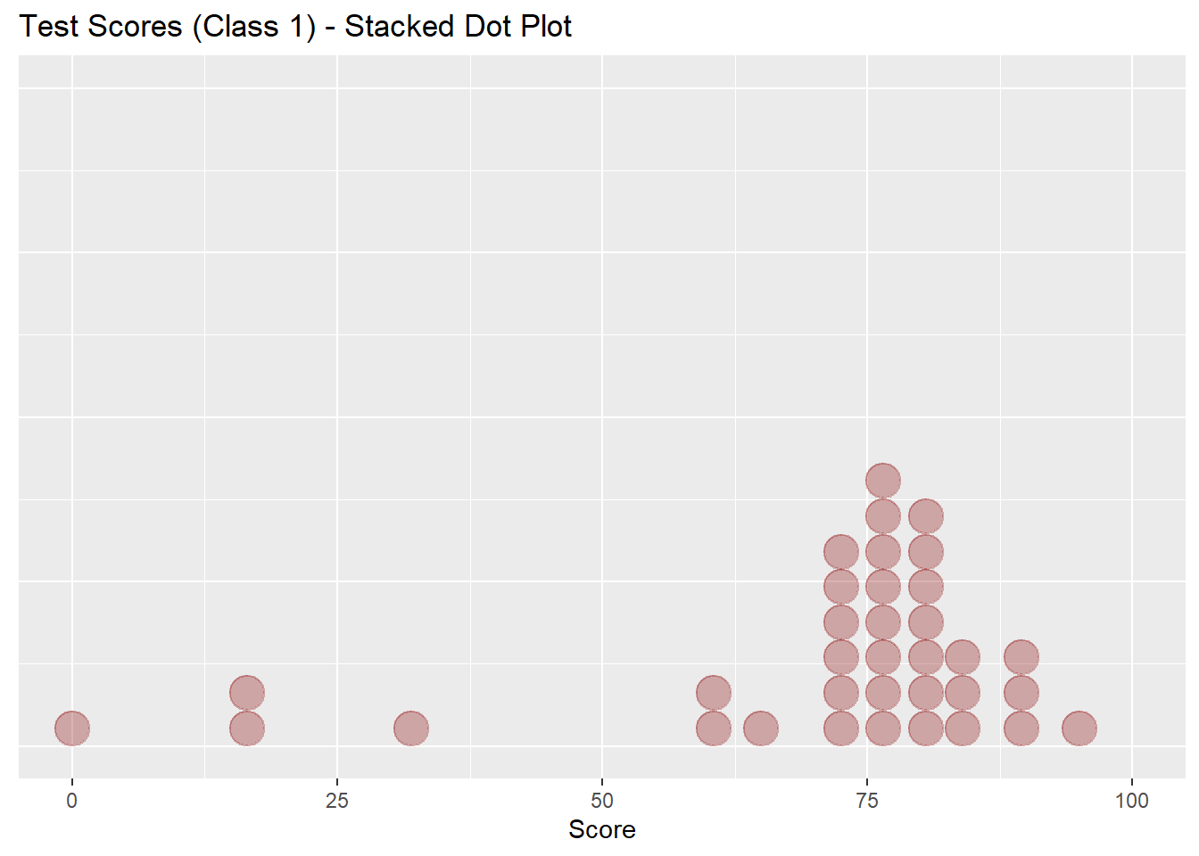
test_scores %>%
    ggplot(aes(x=Score)) +
    geom_dotplot(fill="darkred", color="darkred", alpha = 0.3) +
    xlim(0,100) +
    theme(axis.title.y=element_blank(),
          axis.text.y=element_blank(),
          axis.ticks.y=element_blank()) +
    labs(title = "Test Scores (Classes 1-3) - Stacked Dot Plot")
## `stat_bindot()` using `bins = 30`. Pick better value with `binwidth`.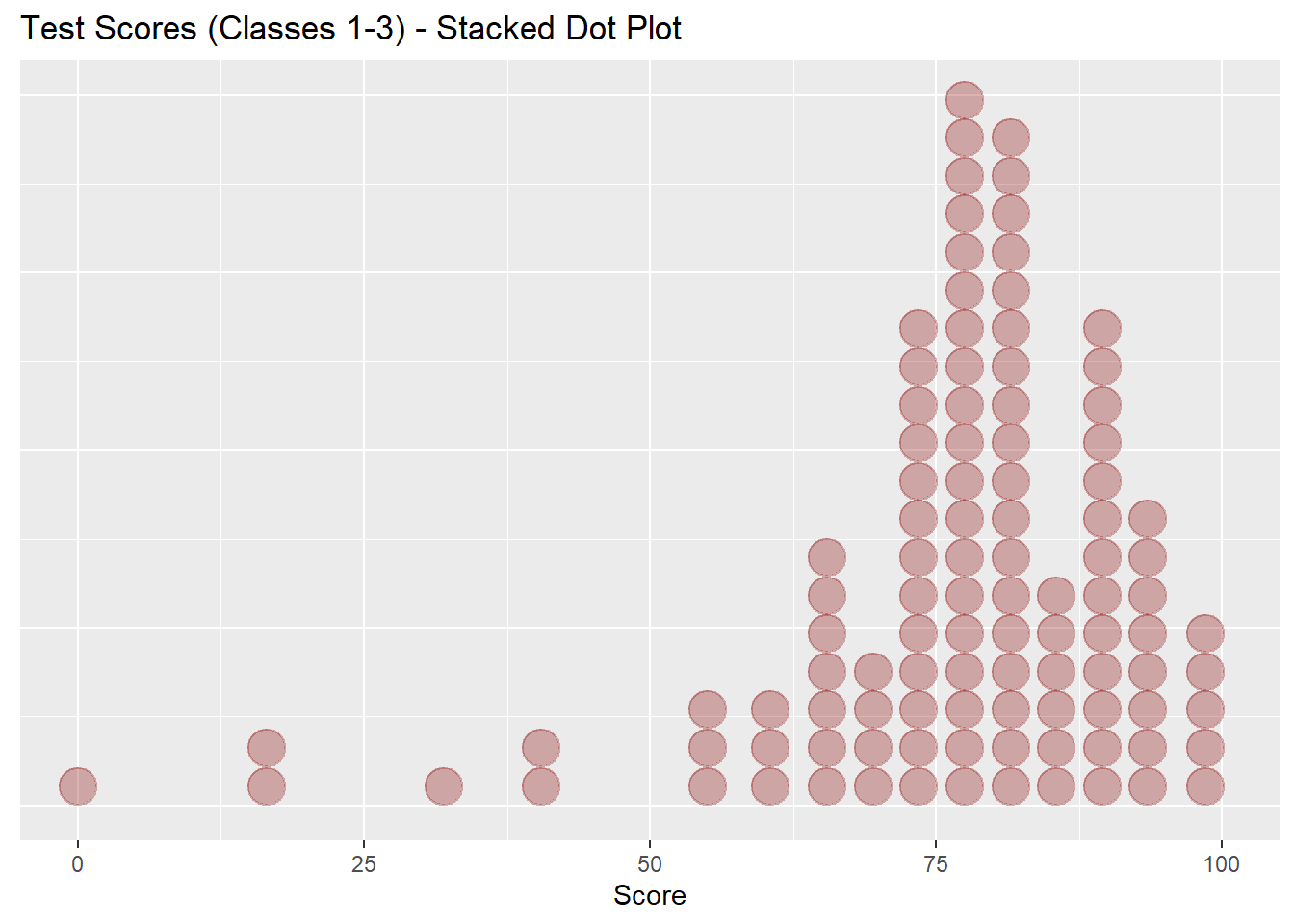
This is not practical when the number of observations in the dataset is large!
Instead, use a histogram:
ggplot(data = test_scores) + geom_histogram(aes(x = Score), bins = 30, fill = "darkred") +
                              labs(title = "Test Scores (All) - Histogram")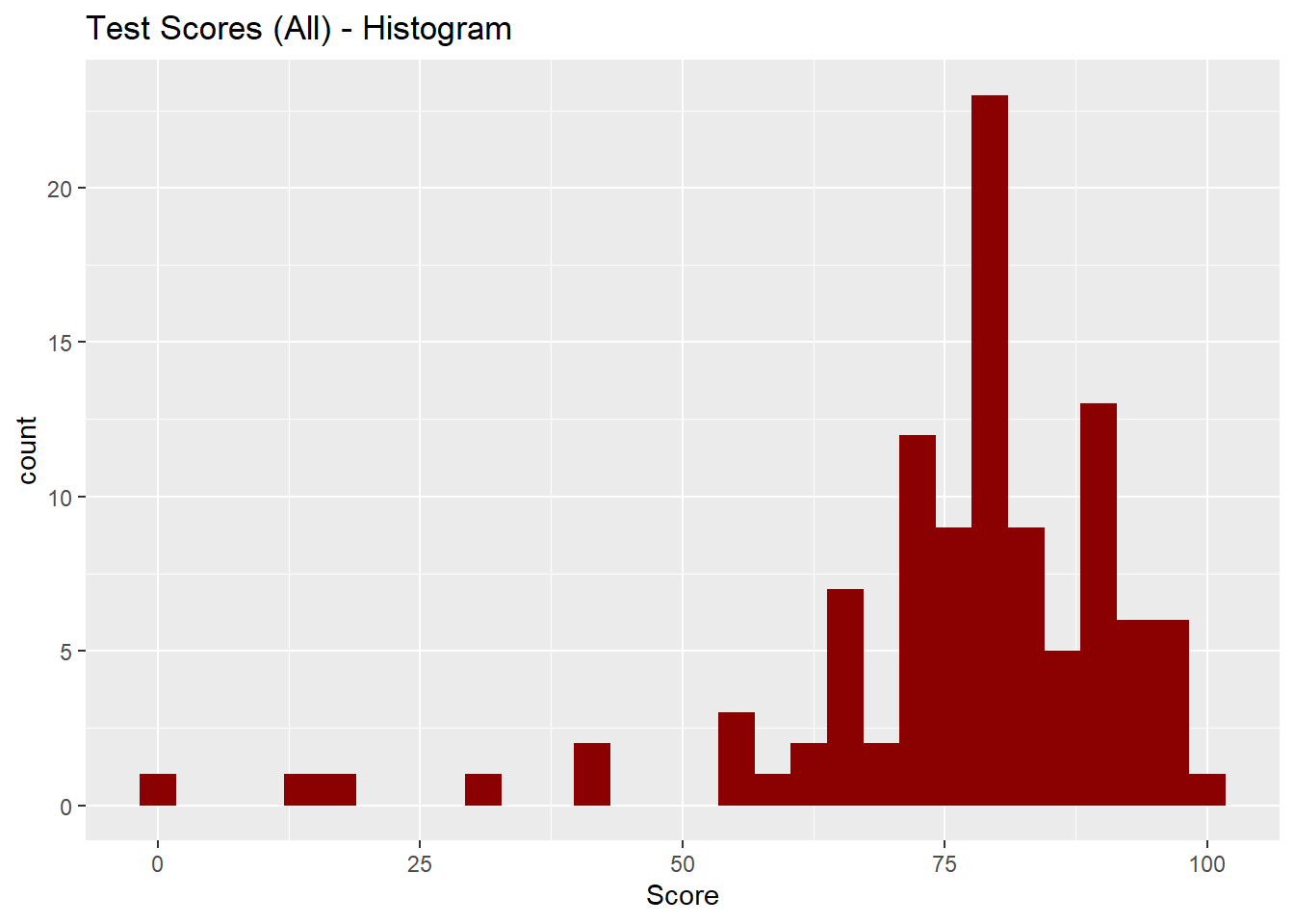
ggplot(data = test_scores) + geom_histogram(aes(x = Score, fill = Class)) +
                             labs(title = "Test Scores (All) - Histogram")
## `stat_bin()` using `bins = 30`. Pick better value with `binwidth`.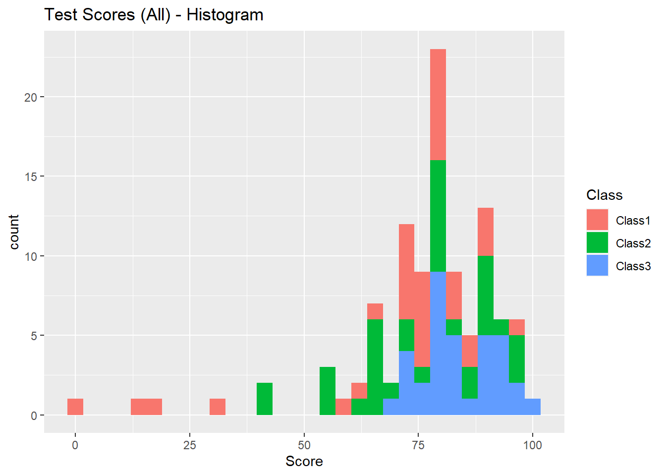
ggplot(data = test_scores) + geom_histogram(aes(x = Score, fill = Class)) + facet_grid(Class ~ .) +
                             labs(title = "Test Scores (Classes 1-3) - Histogram")
## `stat_bin()` using `bins = 30`. Pick better value with `binwidth`.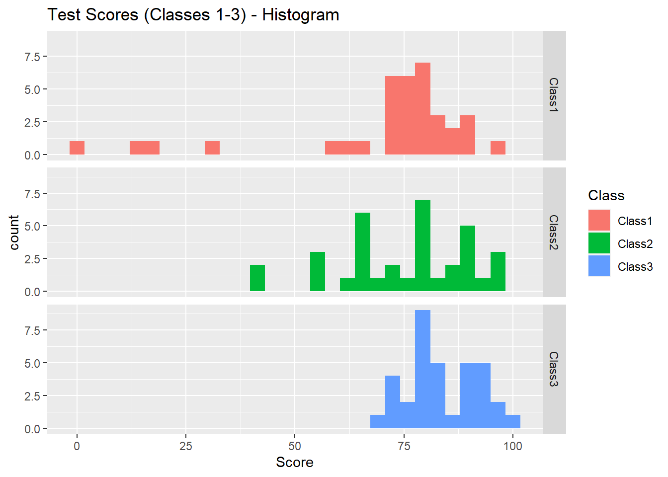
For categorical (nominal or ordinal) variables, use bar charts:
gss98 %>% ggplot() + geom_bar( aes(x = PREMARSX), fill = "darkred" )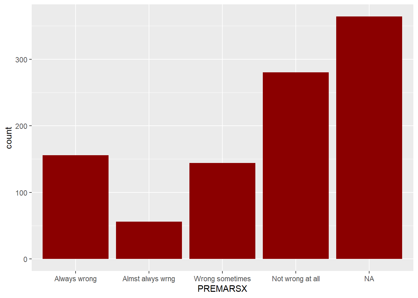
Same, but but without missing values:
gss98 %>% filter(!is.na(PREMARSX)) %>% ggplot() + geom_bar( aes(x = PREMARSX), fill = "darkred" )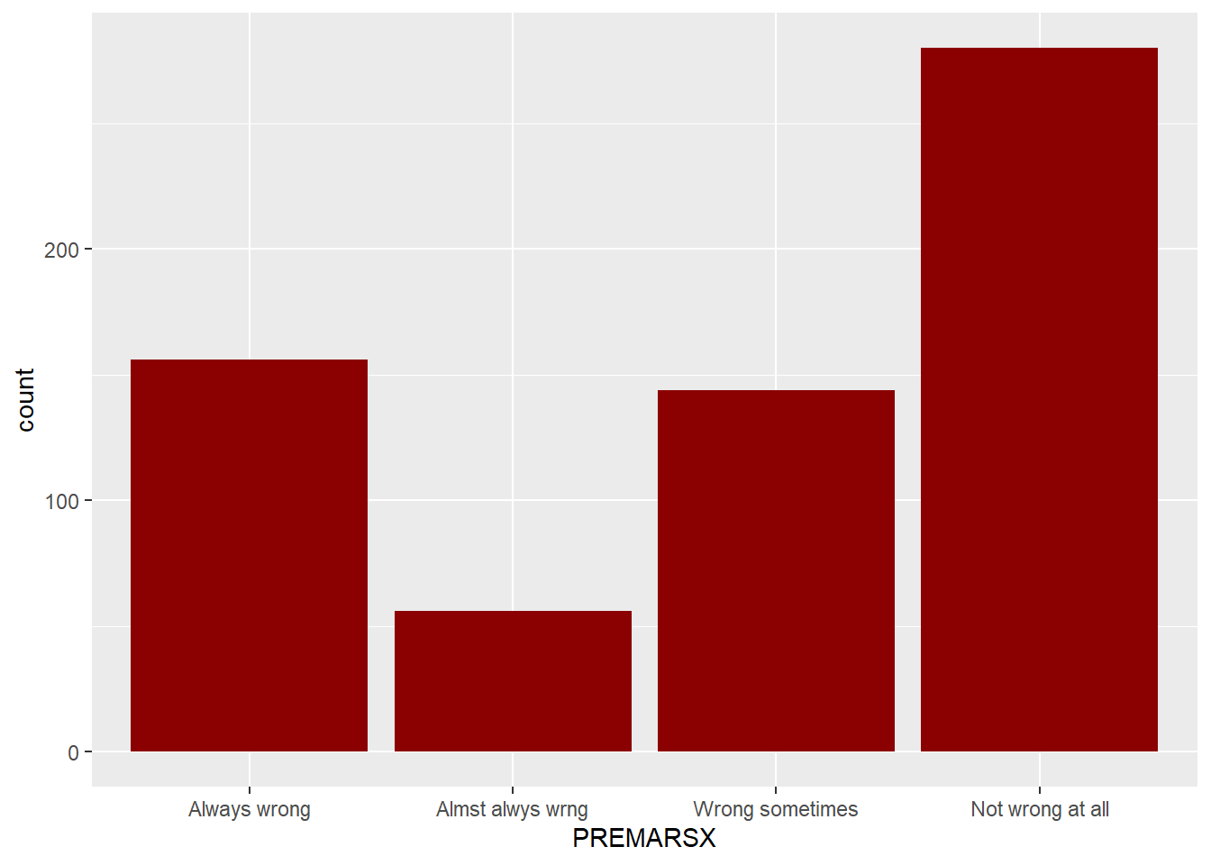
#library(tidyr)
#gss98 %>% tidyr::drop_na(PREMARSX) %>% ggplot() + geom_bar( aes(x = PREMARSX), fill = "darkred" )
Bar plot with relative frequencies and value labels:
gss98 %>%  group_by(PREMARSX) %>% summarise(Percent = 100*n()/nrow(gss98)) %>%  # Calculate % for PREMARSX
    ggplot( mapping = aes(x = PREMARSX, y = Percent, label = Percent)) +        # Map aesthetics
    geom_bar( stat="identity", fill = "darkred" ) +                             # added stat="identity"
    geom_text(vjust = -0.2)                                                     # adjust height of the labels
## Warning: Factor `PREMARSX` contains implicit NA, consider using
## `forcats::fct_explicit_na`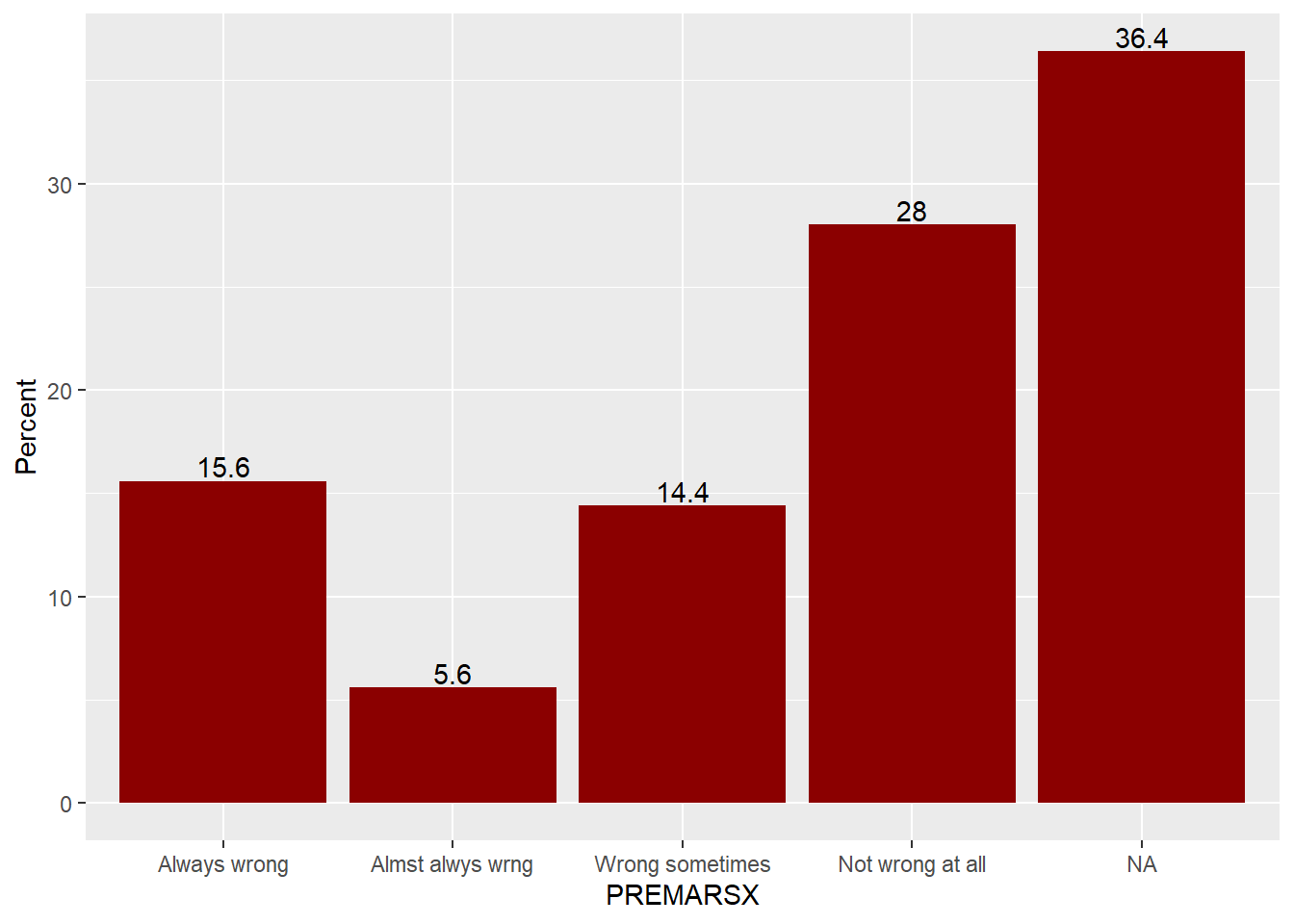
Selected Variables from a random sample of 500 observations from the 2000 U.S. Census Data:
census_year- Census Year.state_fips_code- Name of state.total_family_income- Total family income (in U.S. dollars).age- Age.sex- Sex with levels Female and Male.race_general- Race with levels American Indian or Alaska Native, Black, Chinese, Japanese, Other Asian or Pacific Islander, Two major races, White and * Other.marital_status- Marital status with levels Divorced, Married/spouse absent, Married/spouse present, Never married/single, Separated and Widowed.total_personal_income- Total personal income (in U.S. dollars).
census <- read.csv("C:/Users/admin/Dropbox/PhD/00_Coursework/13sem_4041_Spring2020/R/Datasets/census.csv")
library(summarytools)
Frequency distributions for census$marital_status:
freq(census$marital_status) %>% kable(digits = 2)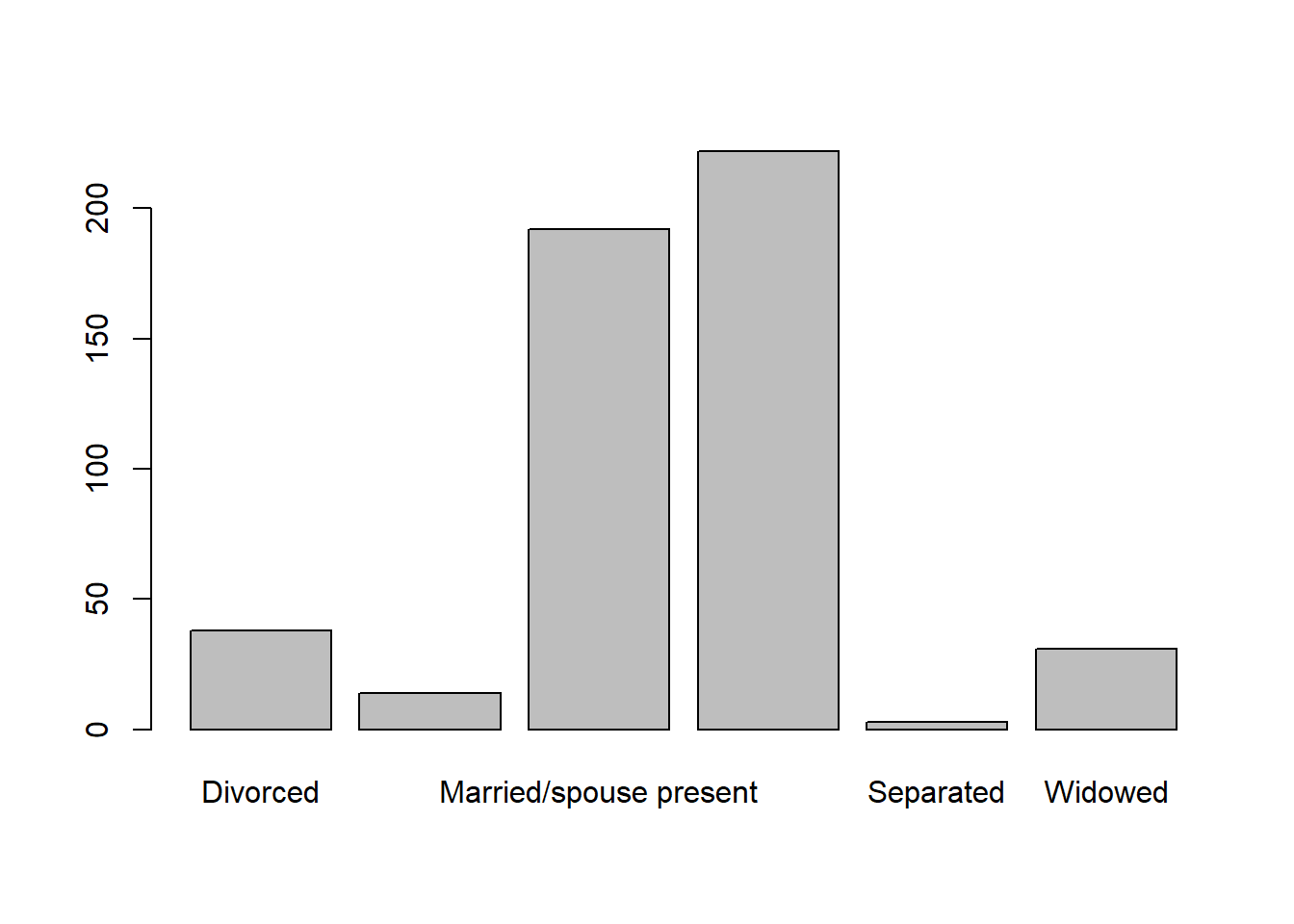
| Frequency | Percent | |
|---|---|---|
| Divorced | 38 | 7.6 |
| Married/spouse absent | 14 | 2.8 |
| Married/spouse present | 192 | 38.4 |
| Never married/single | 222 | 44.4 |
| Separated | 3 | 0.6 |
| Widowed | 31 | 6.2 |
| Total | 500 | 100.0 |
ggplot(data = census) + geom_bar(mapping = aes(x = marital_status)) + theme(axis.text.x = element_text(angle = 45, hjust = 1))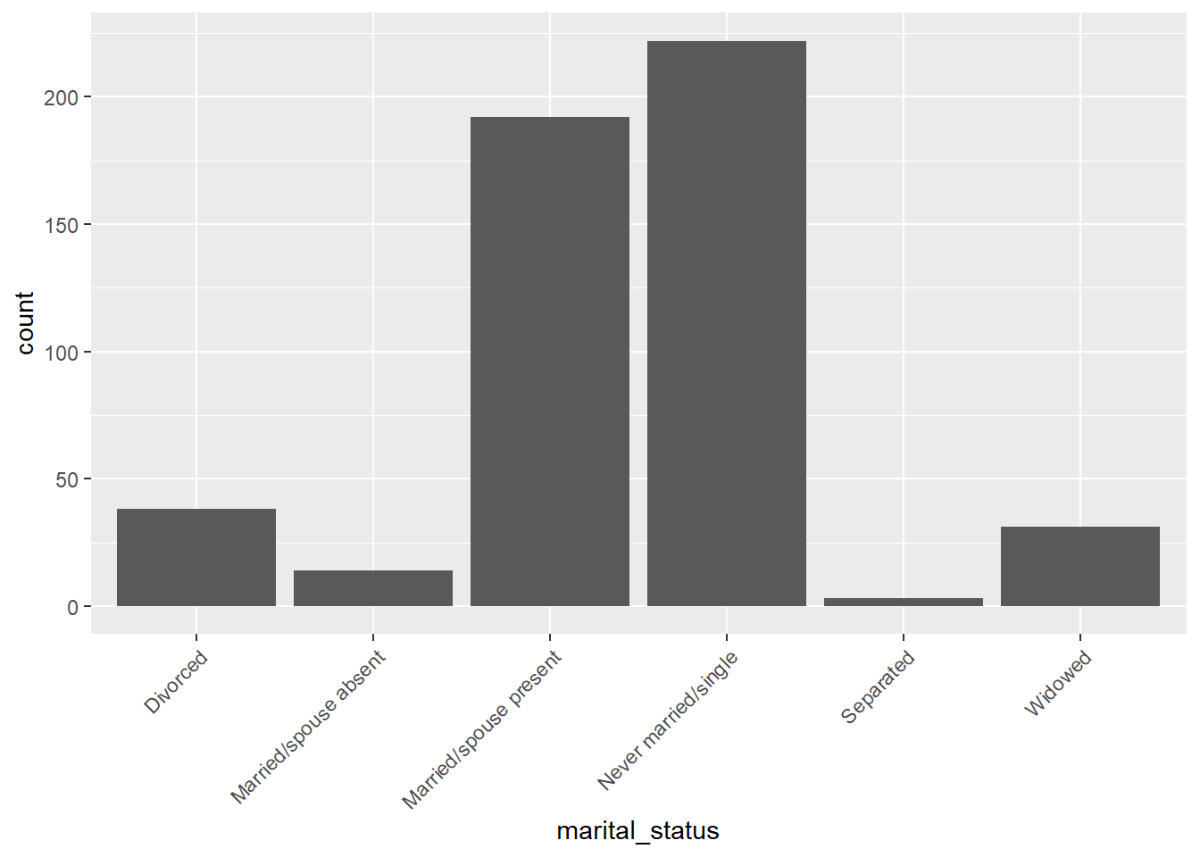
Frequency distributions for census$total_family_income:
income_intervals <- cut(x = census$total_family_income/1000, breaks = c(0,25,50,75,100,999), include.lowest = TRUE)
summarytools::freq(income_intervals)
## Frequencies
##
## Freq % Valid % Valid Cum. % Total % Total Cum.
## --------------- ------ --------- -------------- --------- --------------
## [0,25] 148 30.52 30.52 29.60 29.60
## (25,50] 138 28.45 58.97 27.60 57.20
## (50,75] 90 18.56 77.53 18.00 75.20
## (75,100] 48 9.90 87.42 9.60 84.80
## (100,999] 61 12.58 100.00 12.20 97.00
## <NA> 15 3.00 100.00
## Total 500 100.00 100.00 100.00 100.00ggplot(data = census) + geom_histogram(mapping = aes(x = total_family_income/1000)) + xlab("Total Family Income (Thousands $)")## `stat_bin()` using `bins = 30`. Pick better value with `binwidth`.## Warning: Removed 15 rows containing non-finite values (stat_bin).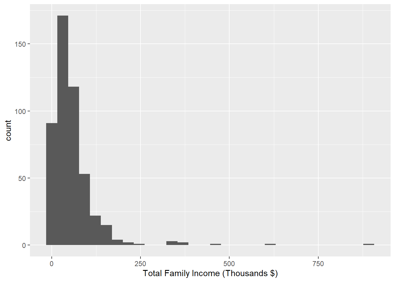
Download the datasets for this class: