Describing Distributions with Numbers (In-class practice)

Download the datasets for this class:

You can download this whole script as week03.Rmd file to save on your computer and open in RStudio instead of copying & pasting from this webpage:

Week #3: Download link - Rmd file - (Click “Save As”)

For those who prefer to work with RCloud, a project with the same materials can be accessed using the following link:

RCloud Project for Week 4/Computer Assignment 3

Load Libraries, Set Your Working Directory, & Load Data

Load Libraries:

library(dplyr)         # for manipulating data
library(ggplot2)       # for making graphs
library(knitr)         # for nicer table formatting
library(summarytools)  # for frequency distribution tables & summary statistics
library(descr)         # for summary statistics

Set working directory, where the folder “Datasets” is located:

setwd(".")             # for example: setwd("C:/Users/George/Dropbox/GSU/4041_Spring2020/R")

Load Data

We are going to work with a new data set - a random sample of 1,000 federal personnel records for March 1994. These are not the responses to questionnaires as the previous data set was. Instead, they include the sort of information the government keeps in its personnel files: grade, salary, occupation, supervisory status, education, age, years of federal experience, sex, race, etc.

load("Datasets/OPM94.RData")

Exploring Dataset

See a full listing of the variables by using names(dataset_name) command and the structure of the dataset using str(dataset_name) :

names(opm94)

##  [1] "x"        "sal"      "grade"    "patco"    "major"    "age"     
##  [7] "male"     "vet"      "handvet"  "hand"     "yos"      "edyrs"   
## [13] "promo"    "exit"     "supmgr"   "race"     "minority" "grade4"  
## [19] "promo01"  "supmgr01" "male01"   "exit01"   "vet01"

str(opm94)

## 'data.frame':    1000 obs. of  23 variables:
##  $ x       : int  1 2 3 4 5 6 7 8 9 10 ...
##  $ sal     : int  26045 37651 64926 18588 19573 28648 27805 16560 40440 24285 ...
##  $ grade   : int  7 9 14 4 3 9 7 3 11 6 ...
##  $ patco   : Factor w/ 5 levels "Administrative",..: 1 4 4 2 2 4 5 2 1 2 ...
##  $ major   : Factor w/ 23 levels "     ","AGRIC",..: 16 11 10 1 1 11 1 1 1 6 ...
##  $ age     : int  52 34 37 26 51 44 50 37 59 57 ...
##  $ male    : Factor w/ 2 levels "female","male": 1 1 1 1 1 1 1 1 1 1 ...
##  $ vet     : Factor w/ 2 levels "no","yes": 1 1 1 1 1 1 1 1 2 1 ...
##  $ handvet : Factor w/ 2 levels "no","yes": 1 1 1 1 1 1 1 1 1 1 ...
##  $ hand    : Factor w/ 2 levels "no","yes": 2 1 1 1 1 1 1 1 1 1 ...
##  $ yos     : int  6 4 3 6 14 1 7 5 13 6 ...
##  $ edyrs   : int  16 16 16 12 12 16 14 12 12 14 ...
##  $ promo   : Factor w/ 2 levels "no","yes": 2 1 1 1 NA 1 1 1 1 1 ...
##  $ exit    : Factor w/ 2 levels "no","yes": 1 1 1 1 2 1 1 1 1 1 ...
##  $ supmgr  : Factor w/ 2 levels "no","yes": 1 1 1 1 1 1 1 1 1 1 ...
##  $ race    : Factor w/ 5 levels "American Indian",..: 2 2 2 2 2 2 2 2 2 2 ...
##  $ minority: int  1 1 1 1 1 1 1 1 1 1 ...
##  $ grade4  : Factor w/ 4 levels "grades 1 to 4",..: 3 4 2 1 1 4 3 1 4 3 ...
##  $ promo01 : num  1 0 0 0 NA 0 0 0 0 0 ...
##  $ supmgr01: num  0 0 0 0 0 0 0 0 0 0 ...
##  $ male01  : num  0 0 0 0 0 0 0 0 0 0 ...
##  $ exit01  : num  0 0 0 0 1 0 0 0 0 0 ...
##  $ vet01   : num  0 0 0 0 0 0 0 0 1 0 ...

See the top ten rows of the dataset and the number of rows (observations) inthe dataset:

head(opm94)

##   x   sal grade          patco major age   male vet handvet hand yos edyrs
## 1 1 26045     7 Administrative LIT    52 female  no      no  yes   6    16
## 2 2 37651     9   Professional HEALT  34 female  no      no   no   4    16
## 3 3 64926    14   Professional ENGR   37 female  no      no   no   3    16
## 4 4 18588     4       Clerical        26 female  no      no   no   6    12
## 5 5 19573     3       Clerical        51 female  no      no   no  14    12
## 6 6 28648     9   Professional HEALT  44 female  no      no   no   1    16
##   promo exit supmgr  race minority          grade4 promo01 supmgr01 male01
## 1   yes   no     no Asian        1   grades 5 to 8       1        0      0
## 2    no   no     no Asian        1  grades 9 to 12       0        0      0
## 3    no   no     no Asian        1 grades 13 to 16       0        0      0
## 4    no   no     no Asian        1   grades 1 to 4       0        0      0
## 5  <NA>  yes     no Asian        1   grades 1 to 4      NA        0      0
## 6    no   no     no Asian        1  grades 9 to 12       0        0      0
##   exit01 vet01
## 1      0     0
## 2      0     0
## 3      0     0
## 4      0     0
## 5      1     0
## 6      0     0

nrow(opm94)

## [1] 1000

Let’s explore salary in this sample:

Histograms

# Histogram using base graphics:
hist(opm94$sal)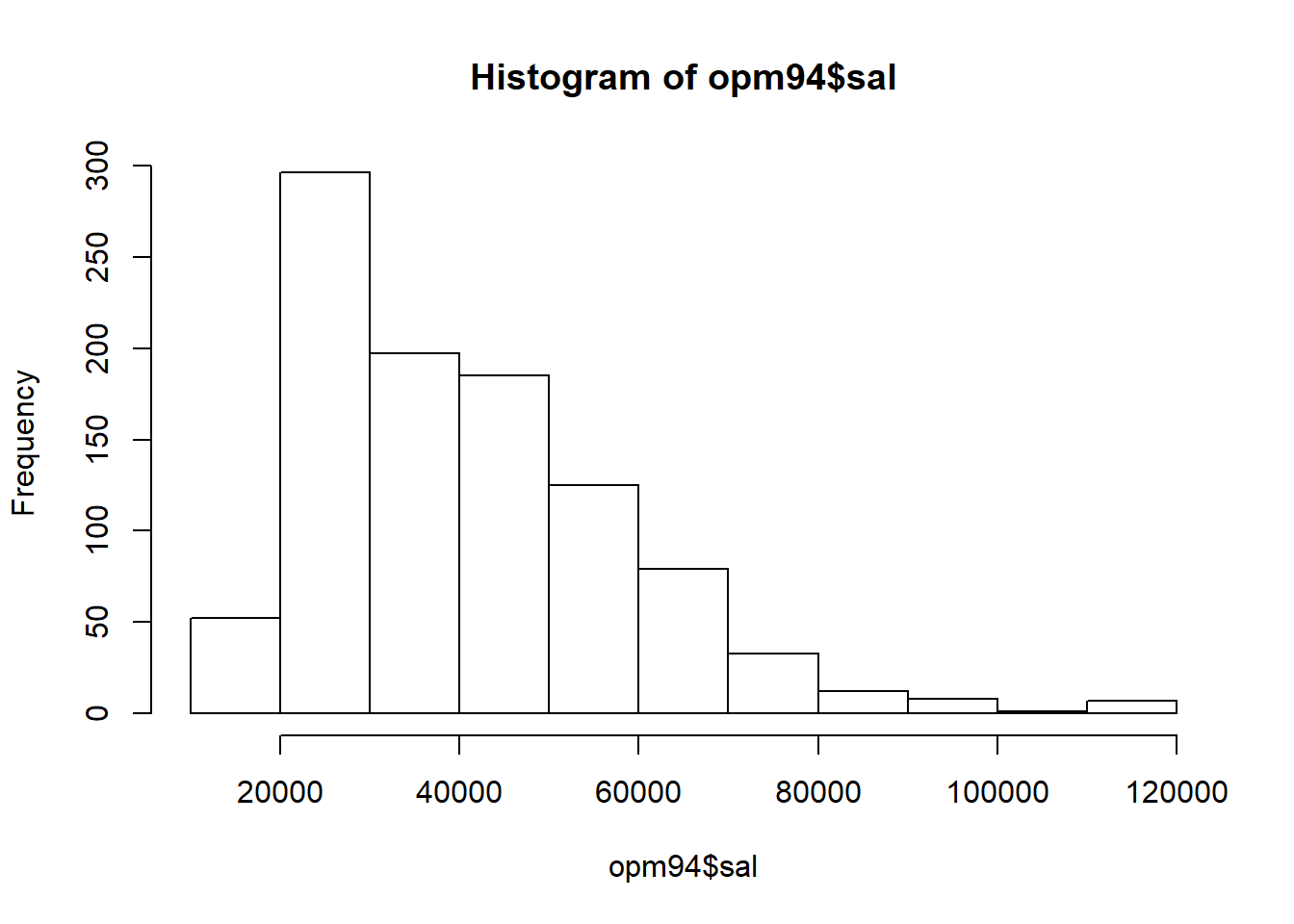

# Histogram using ggplot:
ggplot(data = opm94, aes(x = sal)) + geom_histogram()

## `stat_bin()` using `bins = 30`. Pick better value with `binwidth`.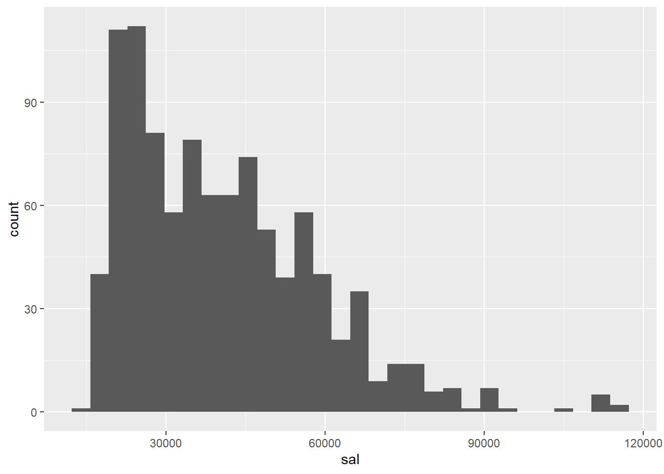

Boxplots

opm94 %>% ggplot( aes(y = sal) ) + geom_boxplot()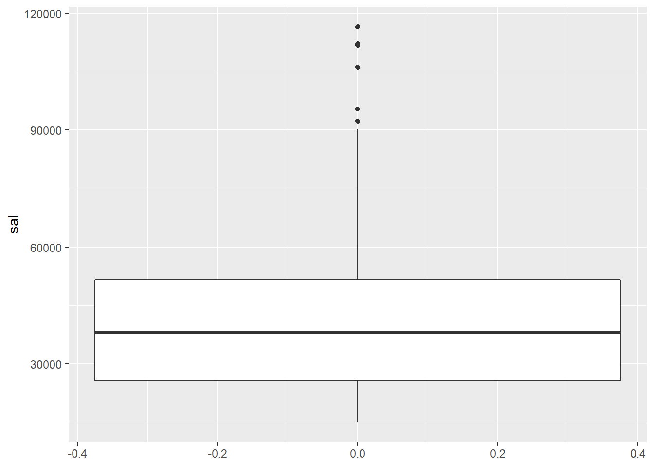

Same plots arranged side-by-side:

plot1 <- ggplot(data = opm94, aes(x = sal)) + geom_histogram()
plot2 <- ggplot(data = opm94, aes(y = sal) ) + geom_boxplot() + coord_flip()

gridExtra::grid.arrange(plot1, plot2, ncol = 1)

## `stat_bin()` using `bins = 30`. Pick better value with `binwidth`.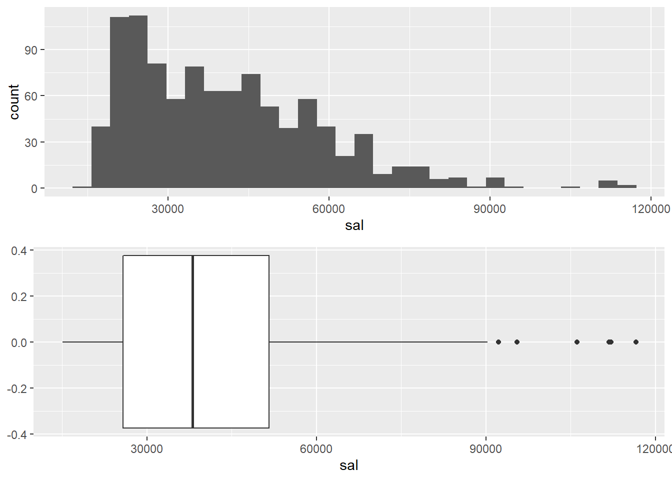

Histograms and boxplots again (across super manager status):

opm94 %>% ggplot( aes(x = supmgr, y = sal) ) + geom_boxplot()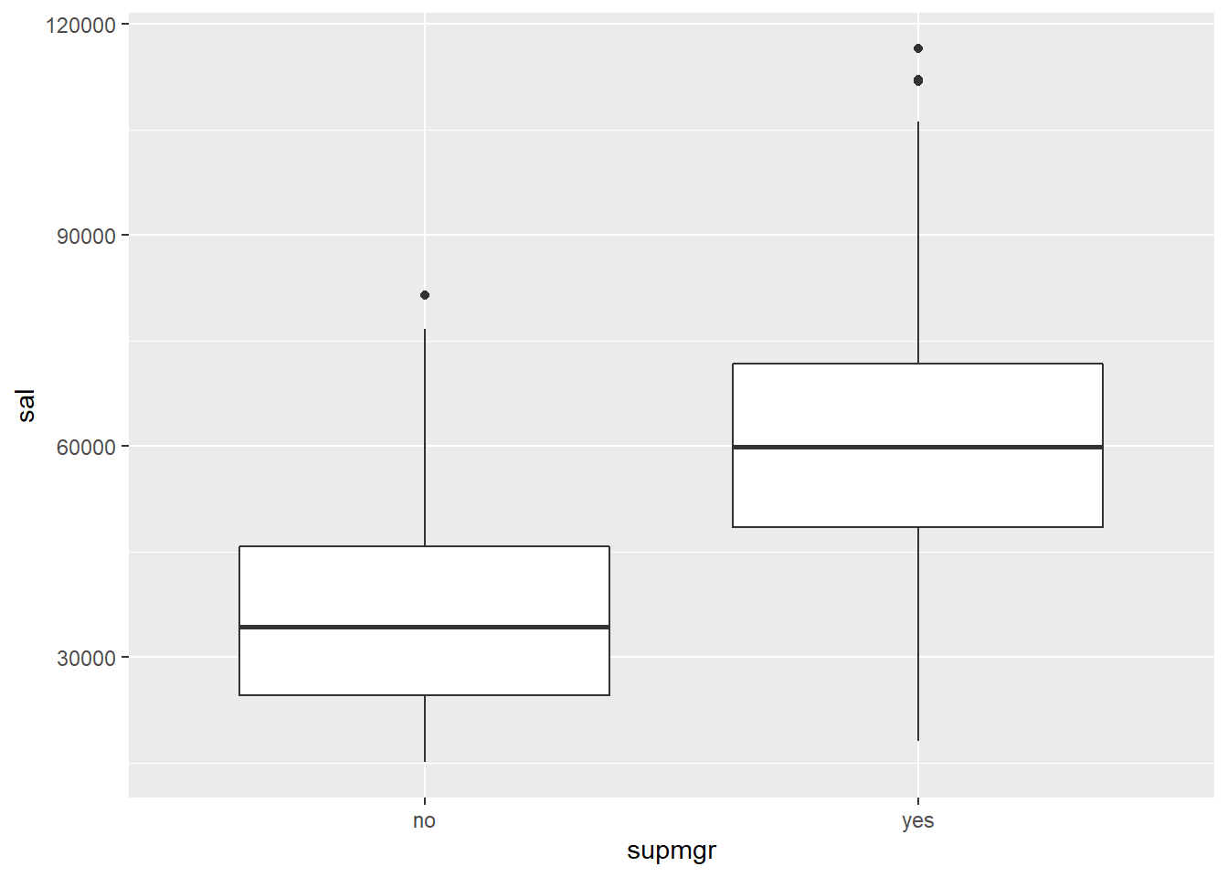

ggplot(data = opm94, aes(x = sal, fill = supmgr)) + geom_histogram() + facet_grid(supmgr ~ .)

## `stat_bin()` using `bins = 30`. Pick better value with `binwidth`.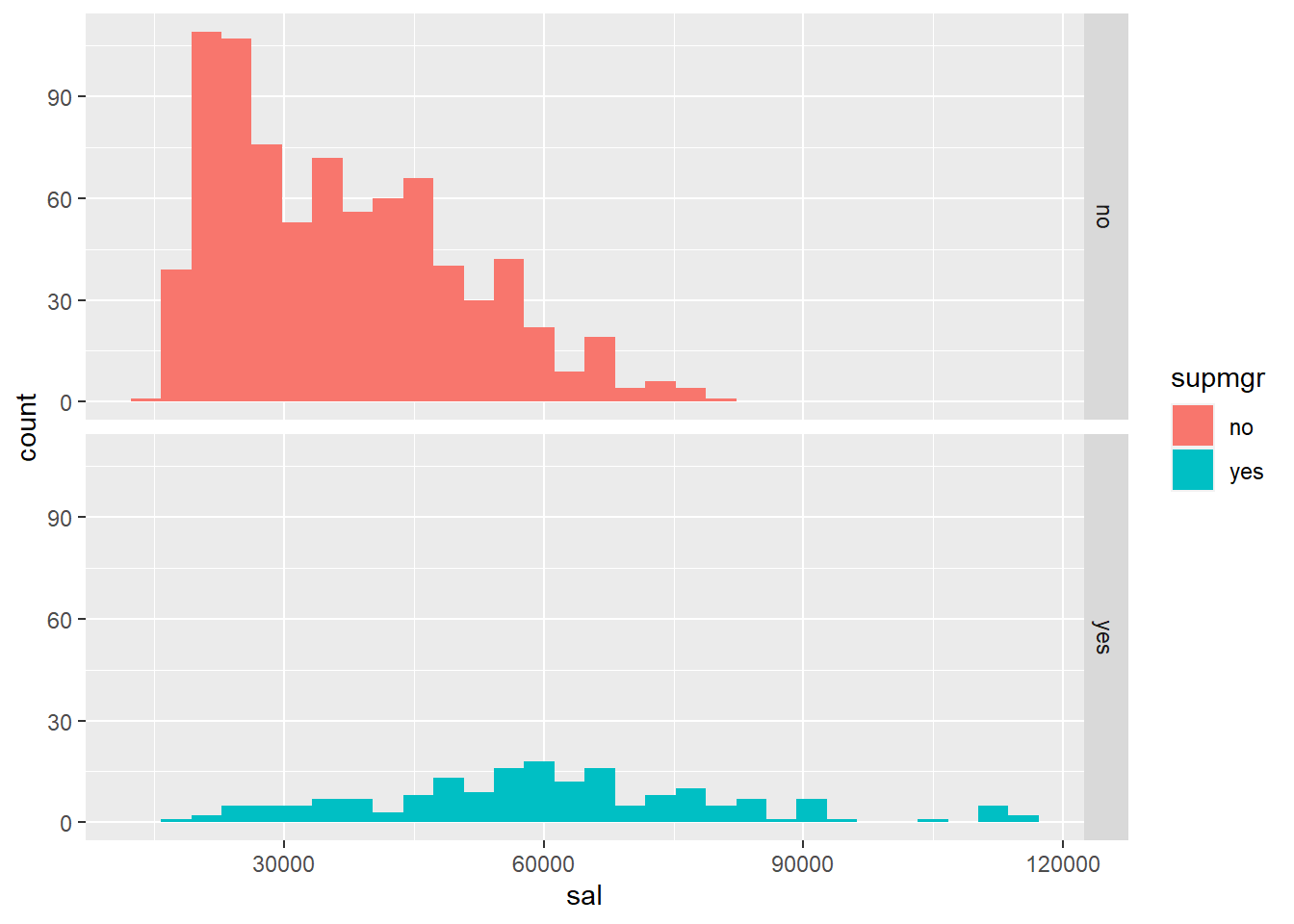

Calculating Statistics

1. Calculating the mode, median, mean, range, variance, and standard deviation

1.1 First, lets work temporarily with American Indian females only (this step will subset the data set): race == "American Indian", male == "female"

opm94AIF <- opm94 %>% filter(race == "American Indian", male == "female")   # subset data
opm94AIF %>% pander::pander(split.table = Inf)                                # print the resulting dataset nicely formatted

x	sal	grade	patco	major	age	male	vet	handvet	hand	yos	edyrs	promo	exit	supmgr	race	minority	grade4	promo01	supmgr01
256	49401	13	Administrative		42	female	no	no	no	14	13	no	no	yes	American Indian	1	grades 13 to 16	0	1
257	25672	5	Technical		31	female	no	no	no	6	13	no	no	no	American Indian	1	grades 5 to 8	0	0
258	23316	5	Clerical		46	female	no	no	no	16	12	no	no	no	American Indian	1	grades 5 to 8	0	0
259	45697	12	Administrative		53	female	no	no	yes	23	15	no	no	yes	American Indian	1	grades 9 to 12	0	1
260	45383	9	Professional		57	female	no	no	no	36	12	no	no	no	American Indian	1	grades 9 to 12	0	0
261	24576	5	Technical		62	female	no	no	no	38	10	no	no	no	American Indian	1	grades 5 to 8	0	0
262	20166	5	Clerical		33	female	no	no	no	6	13	no	no	no	American Indian	1	grades 5 to 8	0	0
263	42751	11	Professional	PUBAF	43	female	no	no	no	16	18	no	no	no	American Indian	1	grades 9 to 12	0	0
264	24585	6	Administrative		53	female	no	no	no	18	15	yes	no	no	American Indian	1	grades 5 to 8	1	0
265	20796	5	Technical		32	female	no	no	no	10	13	no	no	no	American Indian	1	grades 5 to 8	0	0

Let’s print out the individual values of the variables age, edyrs, grade, promo01, supmgr01 in the subset of the data, so that you could calculate statistics manually. We’ll also have the computer calculate the same statistics so that you could check your answers.

Individual values:

opm94AIF <- opm94AIF %>% select("age", "edyrs", "grade", "promo01", "supmgr01")
opm94AIF

##    age edyrs grade promo01 supmgr01
## 1   42    13    13       0        1
## 2   31    13     5       0        0
## 3   46    12     5       0        0
## 4   53    15    12       0        1
## 5   57    12     9       0        0
## 6   62    10     5       0        0
## 7   33    13     5       0        0
## 8   43    18    11       0        0
## 9   53    15     6       1        0
## 10  32    13     5       0        0

Descriptive statistics for the same variables (three different commands/packages to choose from):

Using summary() from base package:

opm94AIF %>% select("age", "edyrs", "grade", "promo01", "supmgr01") %>% summary()

##       age            edyrs           grade         promo01       supmgr01  
##  Min.   :31.00   Min.   :10.00   Min.   : 5.0   Min.   :0.0   Min.   :0.0  
##  1st Qu.:35.25   1st Qu.:12.25   1st Qu.: 5.0   1st Qu.:0.0   1st Qu.:0.0  
##  Median :44.50   Median :13.00   Median : 5.5   Median :0.0   Median :0.0  
##  Mean   :45.20   Mean   :13.40   Mean   : 7.6   Mean   :0.1   Mean   :0.2  
##  3rd Qu.:53.00   3rd Qu.:14.50   3rd Qu.:10.5   3rd Qu.:0.0   3rd Qu.:0.0  
##  Max.   :62.00   Max.   :18.00   Max.   :13.0   Max.   :1.0   Max.   :1.0

Using descr() from descr package:

descr::descr(opm94AIF)

## 
## age
##    Min. 1st Qu.  Median    Mean 3rd Qu.    Max. 
##   31.00   35.25   44.50   45.20   53.00   62.00 
## 
## edyrs
##    Min. 1st Qu.  Median    Mean 3rd Qu.    Max. 
##   10.00   12.25   13.00   13.40   14.50   18.00 
## 
## grade
##    Min. 1st Qu.  Median    Mean 3rd Qu.    Max. 
##     5.0     5.0     5.5     7.6    10.5    13.0 
## 
## promo01
##    Min. 1st Qu.  Median    Mean 3rd Qu.    Max. 
##     0.0     0.0     0.0     0.1     0.0     1.0 
## 
## supmgr01
##    Min. 1st Qu.  Median    Mean 3rd Qu.    Max. 
##     0.0     0.0     0.0     0.2     0.0     1.0

Using descr() from summarytools package:

summarytools::descr(opm94AIF)

## Descriptive Statistics  
## 
##                        age    edyrs    grade   promo01   supmgr01
## ----------------- -------- -------- -------- --------- ----------
##              Mean    45.20    13.40     7.60      0.10       0.20
##           Std.Dev    10.97     2.17     3.31      0.32       0.42
##               Min    31.00    10.00     5.00      0.00       0.00
##                Q1    33.00    12.00     5.00      0.00       0.00
##            Median    44.50    13.00     5.50      0.00       0.00
##                Q3    53.00    15.00    11.00      0.00       0.00
##               Max    62.00    18.00    13.00      1.00       1.00
##               MAD    14.83     1.48     0.74      0.00       0.00
##               IQR    17.75     2.25     5.50      0.00       0.00
##                CV     0.24     0.16     0.44      3.16       2.11
##          Skewness     0.02     0.59     0.53      2.28       1.28
##       SE.Skewness     0.69     0.69     0.69      0.69       0.69
##          Kurtosis    -1.62    -0.29    -1.66      3.57      -0.37
##           N.Valid    10.00    10.00    10.00     10.00      10.00
##         Pct.Valid   100.00   100.00   100.00    100.00     100.00

1.2 Using the raw data above, let’s compute (as appropriate) the mode, median, mean, range, variance, and standard deviation for variable age (opm94AIF$age: 42 31 46 53 57 62 33 43 53 32 ) listed for American Indian females:

age <- opm94AIF$age  # save the values in a new variable with the name `age` for less typing

Mode age

table(c(42, 31, 46, 53, 57, 62, 33, 43, 53, 32))    # figure out the mode from the table or use which.max()

## 
## 31 32 33 42 43 46 53 57 62 
##  1  1  1  1  1  1  2  1  1

which.max(table(c(42, 31, 46, 53, 57, 62, 33, 43, 53, 32)))

## 53 
##  7

Median age

sort(c(42, 31, 46, 53, 57, 62, 33, 43, 53, 32)) # find the median from the ordered vector or use R function median()

##  [1] 31 32 33 42 43 46 53 53 57 62

median(opm94AIF$age)

## [1] 44.5

Mean age:

(42+31+46+53+57+62+33+43+53+32)/10        # or

## [1] 45.2

sum(opm94AIF$age)/length(opm94AIF$age)

## [1] 45.2

mean(opm94AIF$age)

## [1] 45.2

Range for age:

sort(c(42, 31, 46, 53, 57, 62, 33, 43, 53, 32))   # or

##  [1] 31 32 33 42 43 46 53 53 57 62

range(opm94AIF$age)

## [1] 31 62

Variance = SSD/(n-1)

age

##  [1] 42 31 46 53 57 62 33 43 53 32

age - mean(age)

##  [1]  -3.2 -14.2   0.8   7.8  11.8  16.8 -12.2  -2.2   7.8 -13.2

(age - mean(age))^2

##  [1]  10.24 201.64   0.64  60.84 139.24 282.24 148.84   4.84  60.84 174.24

sum((age - mean(age))^2)/(10-1)

## [1] 120.4

var(age)

## [1] 120.4

SD = sqrt(var)

sqrt(sum((age - mean(age))^2)/(10-1) )

## [1] 10.97269

sd(age)

## [1] 10.97269

2. Calculating mode, median, mean for grouped data

Let’s generate grouped data (frequency table) that you will use for calculating statistics (mode, median, mean) for variable edyrs from the full dataset opm94:

summarytools::freq(opm94$edyrs)   # grouped data

## Frequencies  
## 
##               Freq   % Valid   % Valid Cum.   % Total   % Total Cum.
## ----------- ------ --------- -------------- --------- --------------
##          10     12      1.20           1.20      1.20           1.20
##          12    330     33.00          34.20     33.00          34.20
##          13    101     10.10          44.30     10.10          44.30
##          14     98      9.80          54.10      9.80          54.10
##          15     39      3.90          58.00      3.90          58.00
##          16    290     29.00          87.00     29.00          87.00
##          18    112     11.20          98.20     11.20          98.20
##          20     18      1.80         100.00      1.80         100.00
##        <NA>      0                               0.00         100.00
##       Total   1000    100.00         100.00    100.00         100.00

summary(opm94$edyrs)  # summary statistics by R

##    Min. 1st Qu.  Median    Mean 3rd Qu.    Max. 
##   10.00   12.00   14.00   14.37   16.00   20.00

Finding mode, median, mean for edyrs using the grouped data:

Mode - the most frequent vaue, can be seen in the frequency table (=12)
Median - the value in the middle, can be seen in the frequency table from the % Valid Cum. column (=14)
Mean: SUM(Xi*fi)/n:

(10*12 + 12*330 + 13*101 + 14*98 + 15*39 + 16*290 + 18*112 + 20*18)/1000

## [1] 14.366

3. Calculating mode, median, mean for grouped data (dummy variables)

QUESTION 3: Male01 and exit01 are dummy variables. (They only have two possible values, o and 1.) For each, compare its mean to the percentage of cases with the value 1. How are these two measures related?

Percentage of cases with the value 0 and 1 for male01:

table(opm94$male01) %>% prop.table()*100

## 
##    0    1 
## 48.8 51.2

Mean value of male01:

mean(opm94$male01)

## [1] 0.512

4. Calcualting the mean for grouped data formulas for intervals

Using the Frequencies output for the entire data set (and the grouped data formulas for intervals), let’s calculate the mean grade, using grade4 instead of grade using the midpoint of each interval of grade4

summarytools::freq(opm94$grade4)

## Frequencies  
## 
##                         Freq   % Valid   % Valid Cum.   % Total   % Total Cum.
## --------------------- ------ --------- -------------- --------- --------------
##         grades 1 to 4     70      7.00           7.00      7.00           7.00
##       grades 13 to 16    223     22.30          29.30     22.30          29.30
##         grades 5 to 8    299     29.90          59.20     29.90          59.20
##        grades 9 to 12    408     40.80         100.00     40.80         100.00
##                  <NA>      0                               0.00         100.00
##                 Total   1000    100.00         100.00    100.00         100.00

5. Comparing means for different groups

Let’s calculate mmeans of a variety of variables for black and white workers so that you can describe differences between the two groups of workers:

opm94$race %>% table()

## .
## American Indian           Asian           Black        Hispanic           White 
##              17              31             175              49             728

opm94 %>% filter(race == "White") %>% select(sal) %>% summarise(mean_sal_white = mean(sal, na.rm = T))

##   mean_sal_white
## 1       43294.39

opm94 %>% filter(race == "Black") %>% select(sal) %>% summarise(mean_sal_black = mean(sal, na.rm = T))

##   mean_sal_black
## 1       32712.78

# Or, alternatively, use: 
opm94 %>% select(race, sal) %>% group_by(race) %>% summarise(mean_sal = mean(sal, na.rm = T))

## # A tibble: 5 x 2
##   race            mean_sal
##   <fct>              <dbl>
## 1 American Indian   32846.
## 2 Asian             38440.
## 3 Black             32713.
## 4 Hispanic          36500.
## 5 White             43294.

opm94 %>% select(race, grade) %>% group_by(race) %>% summarise(mean_grade = mean(grade, na.rm = T))

## # A tibble: 5 x 2
##   race            mean_grade
##   <fct>                <dbl>
## 1 American Indian       8.24
## 2 Asian                 9.65
## 3 Black                 7.91
## 4 Hispanic              8.94
## 5 White                10.1

opm94 %>% select(race, promo01) %>% group_by(race) %>%  summarise(mean_promo01 = mean(promo01, na.rm = T))

## # A tibble: 5 x 2
##   race            mean_promo01
##   <fct>                  <dbl>
## 1 American Indian        0.25 
## 2 Asian                  0.172
## 3 Black                  0.126
## 4 Hispanic               0.213
## 5 White                  0.123

opm94 %>% select(race, supmgr01) %>% group_by(race) %>%  summarise(mean_supmgr01 = mean(supmgr01, na.rm = T))

## # A tibble: 5 x 2
##   race            mean_supmgr01
##   <fct>                   <dbl>
## 1 American Indian         0.118
## 2 Asian                   0.161
## 3 Black                   0.109
## 4 Hispanic                0.143
## 5 White                   0.201